A circular economy is an economic model that aims to minimize waste and maximize resource efficiency.
It involves designing products and processes focusing on longevity, reuse and recycling.
Why not rent your dress instead of buying it?!
Several fashion retailers have implemented a subscription model.

Customers pay a regular fee to access a product or service for a specific period.
How sustainable is this circular economy model?
The objective is to reduce the environmental impact along products’ life cycles.

Can you use data science to estimate the emissions reduction of an experimental rental model?
We have built a build simulation model to assess the effectiveness of these initiatives.
This article will estimate the environmental impacts of implementing a rental model with 400 items for a fashion retailer.
Circular Rental Models for Fast Fashion
Support the Decarbonization of your Supply Chain
You work with the logistics department of an international clothing group with stores worldwide.
To support the United Nations Sustainable Development Goals, the company has committed to reducing its environmental footprint.
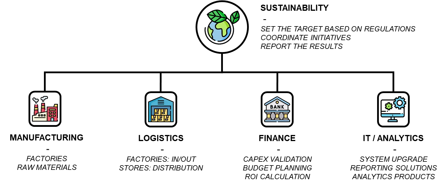
Therefore, your colleagues from the sustainability department prepared a roadmap involving several departments for reducing carbon footprints by 2030.
Among the initiatives, it has been decided to experiment with a circular economy model in 10 stores.
These locations will propose a rental subscription model to their customers for a limited scope of 400 items.
Before implementing this additional service, logistics and sustainability teams requested your support to estimate the emissions cuts we can reach.
Operational Assumptions
The inventory at the store is managed by distribution planners using an ERP.
- Stores are replenished by a Central Warehouse
- Factories replenish the Central Warehouse
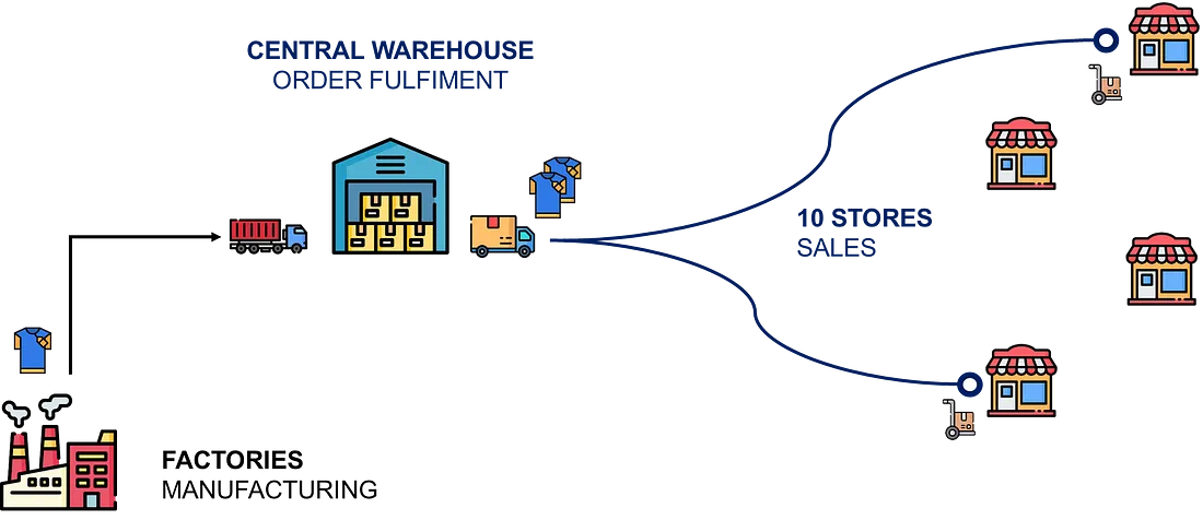
For this simulation, we will use the model designed for the article about Green Inventory Management, considering the following assumptions:
- 365 days of sales transactions in 10 locations
- 3,300 active SKUs with 400 SKUs included in the circular model
- Inventory Periodic Review Policy Rule: 2 days
That means your stores are replenished every two days by the Central Warehouse.
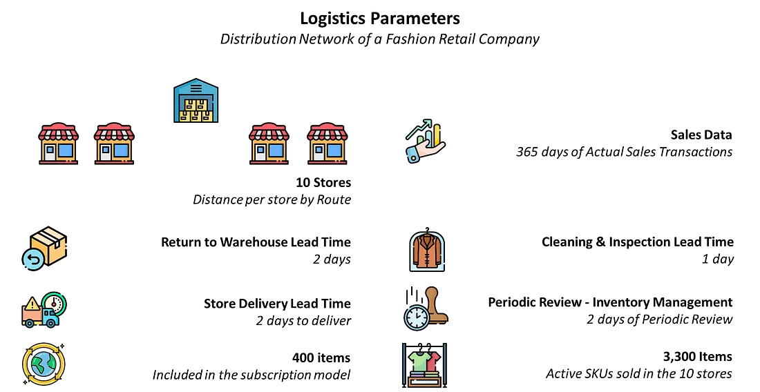
We will add the assumptions linked to the circular model
- Delivery Lead Time from Warehouse for Circular Items: 2 days
- Cleaning & Inspection at Warehouse: 1 day
- Return to Warehouse Lead Time: 2 days
When an item is returned at the end of the rental period, it takes two days to ship it back to the warehouse.
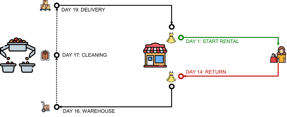
Another day is needed to inspect and clean it.
Finally, it will be returned to a store after two additional days.
Now that we have introduced the assumptions, we can focus on the simulation.
Simulation Model of the Circular Model
The main parameter of our circular model will be the rental period.
What is the optimal rental period to maximize the emissions reductions?
The objective is to test several rental periods to observe the impact on CO2 emissions and water usage reduction.
Inventory Management Model
Unlike a standard linear model, our inventory will include two types of items.
If a customer is renting a dress, she may
- Rent a dress returned by a previous customer (after cleaning).
- Rent a new dress coming from the factory.
I will apply the First-In, First-out (FIFO) principle to orchestrate these flows to every store order.
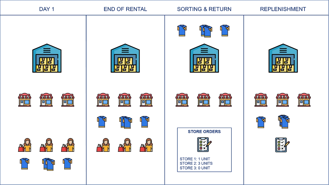
Taking the example above,
- After cleaning and inspection, these four returned items are available for order.
- Store 2 sent the first replenishment order with a quantity of 3 units.
- Store 1 sent later a replenishment order with a quantity of 1 unit.
Because store 2 ordered first, the first three units that arrived in the warehouse stock will be shipped there.
If the returned product inventory is too low, orders are completed with new items.
These additional parameters have been included in the simulation model following the example I presented in this article.
To assess the performance of your circular economy, we focus on the
- Total CO2e emissions of your Supply Chain (kg CO2e)
- Quantity of water used to produce and deliver items to stores (L)
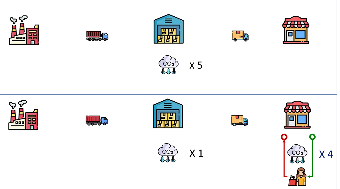
In the example above, we switch from 5 purchases to 5 rentals of this item.
The footprint of the circular model includes
- A single full cycle from raw material extraction to store delivery.
- Four return cycles with reverse logistics and cleaning process.
We can then estimate the savings using the formulas below,
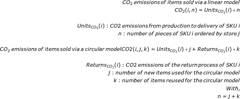
The major assumption behind this approach is that the percentage of items reused will drive the savings.
These formulas should be coupled with life cycle assessment metrics linked to each item in the scope of analysis.
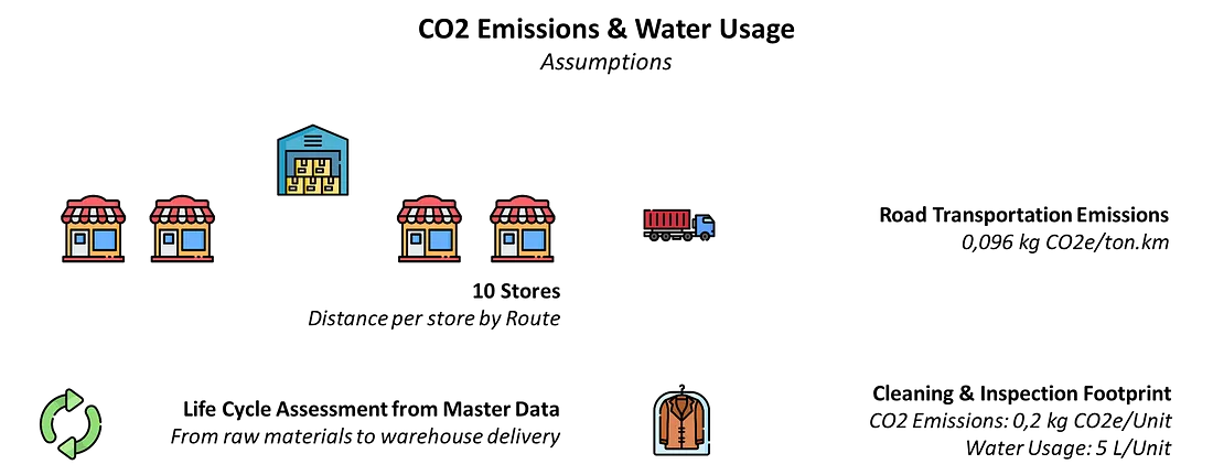
- Emissions and water are taken from the master data.
- The additional impacts are estimated using the parameters listed above.
The remaining parameter that should be defined is the rental duration.
Simulation Scenarios
After discussing this with the merchandising and logistics teams, you have selected potential durations of 2, 7, 14, and 28 days.
You will simulate each scenario's forward and reverse flows using actual sales transactions.
Let us now see the results for these four different rental periods.
Could you guess which period provides the highest emissions (and water usage) reduction?
Simulation for a rental period of 7 days
Now that we have built our model with the right assumptions, we can start exploring the results with a one-week rental period.
The percentage of circularity
What is the percentage of new items used?
💡 Insights
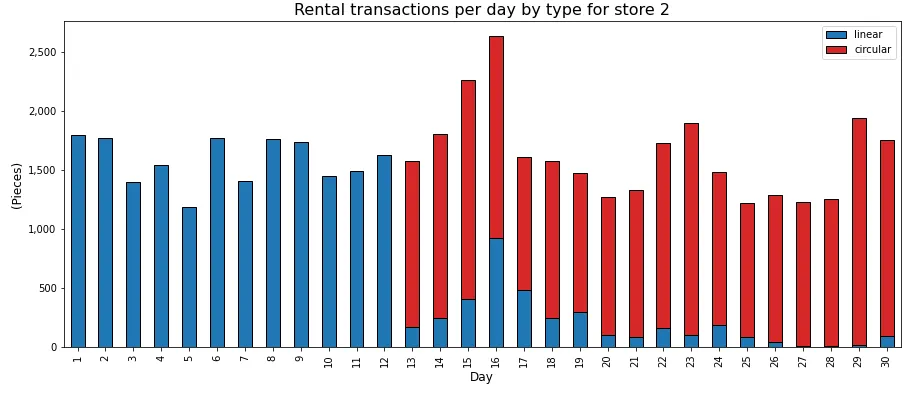
- During the first 12 days, the inventory of returned items is zero, so the store is using only new items for rental.
- When there are volume peaks, like on day 16, the accumulated inventory of returned items cannot meet the demand.
The percentage of circularity (%) is the ratio of returned items for the rental transactions.
This is an important parameter influencing the environmental performance of your circular model.
Your rental model's footprint is highest during the first 12 days as we use new items.
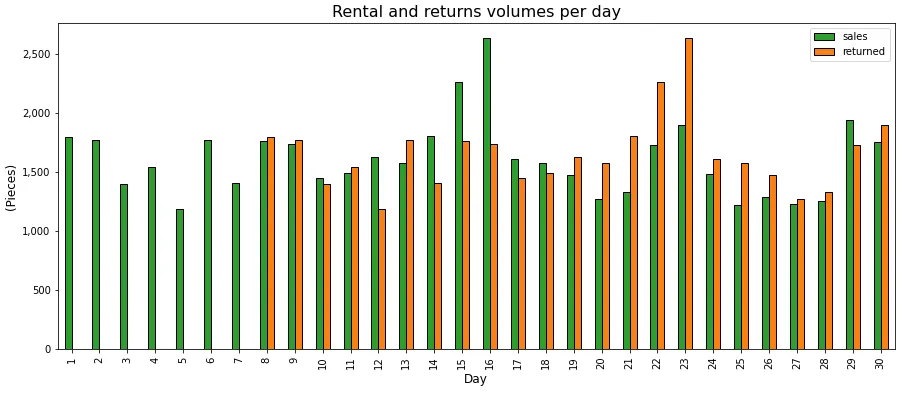
This can be easily explained by looking at the volume of returned items.
Indeed, we can see that the first batch of rented items was returned on the 8th day.
After 5 days for the return process (pick-up, cleaning and store shipping), they are available on day 13 for new sales.
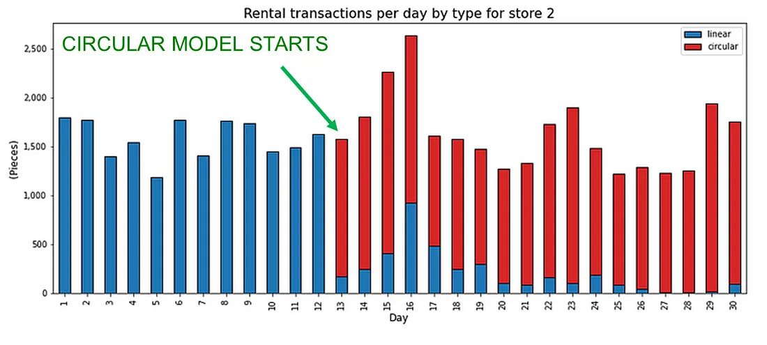
From this day, we have a balanced distribution of rented and returned items to obtain enough inventory to reuse more than 75% of items.
How many times an item is rented on average?
This chart shows the distribution of items by the number of rental cycles along the simulation period.
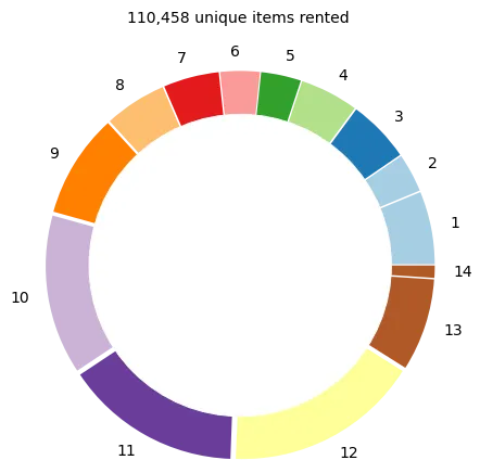
For instance, 9.8% of items have been used 10 times.
💡 Insights
- 110,458 unique items are used to fulfil 951,856 rental transactions
An average of 8.61 rental cycles per item. - Some items can reach 14 cycles.
- A non-negligible part of the inventory is only used a single time.
What is the environemental impact for each item?
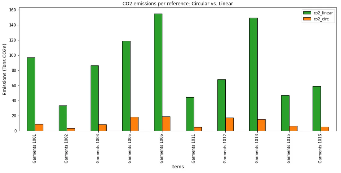
Let us take the example of a coat rented to 35 customers using only 10 unique pieces.
We define the linear model’s emissions (co2_linear in green) as the total footprint if these customers purchased 35 coats items.
The circular model’s emissions (co2_circ in orange) only include the production of 10 unique coats and the logistics for return management.
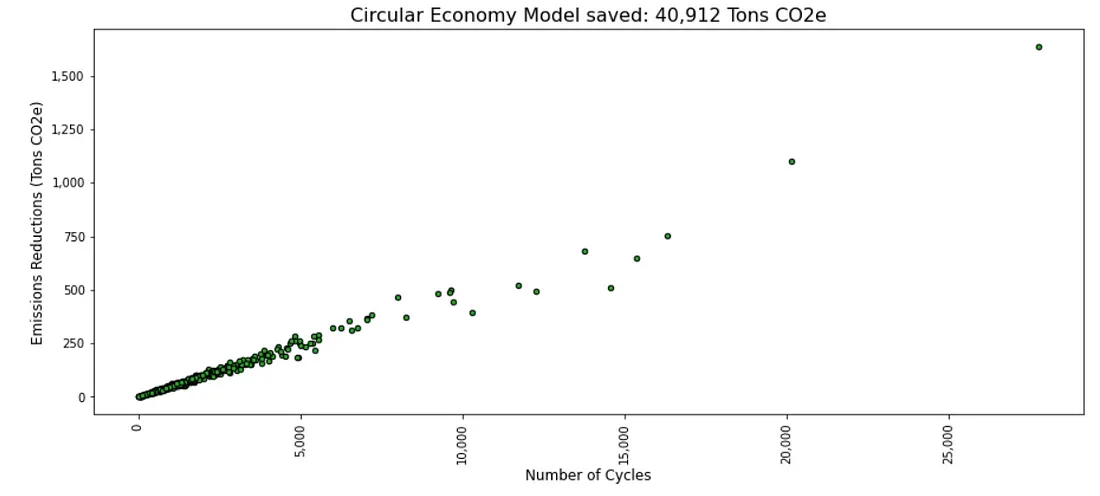
Is there any correlation between emissions reductions and the number of rental cycles?
What is the impact of demand variability?
As expected, the amount of CO2e reduction is linearly linked with the number of cycles.
What does impact the percentage of reused items?
Therefore, we would like to reach 100% of rental transactions with reused items and limit the number of new items purchased.
What influences the percentage of transactions with reused items?
When demand is highly volatile, the inventory of returned items is quickly finished. Therefore, you need to purchase newly produced items.
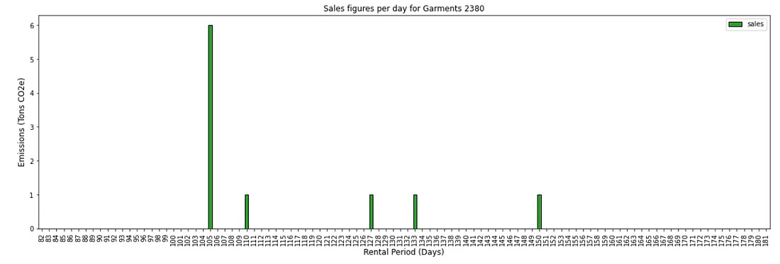
In the example above, the demand distribution is highly skewed.
- 60% of the total demand for this reference occurs at the peak of day 105
- Therefore, the percentage of circularity (number of sales transactions fulfilled with reused items) is only 40%.
What if we have a stable demand?
The bar chart below shows the sales distribution of SKU Garments 1018; this high-runner has a stable distribution.
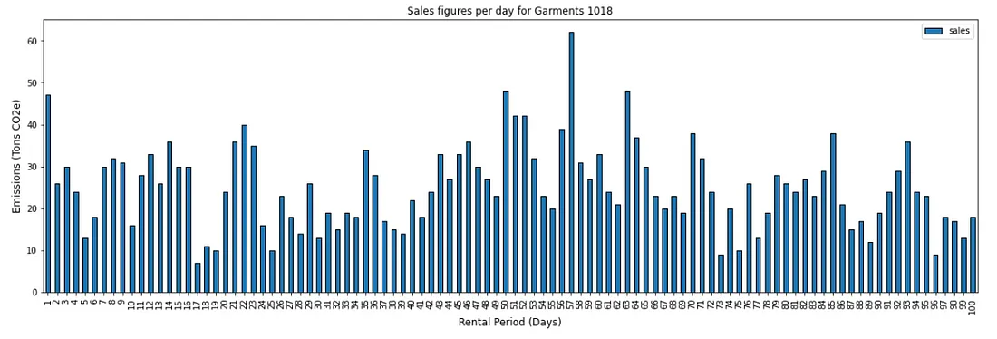
- Except for the first days, the demand distribution provides enough flexibility to build an inventory of returned products.
- Therefore, we can reach 89% of sales transactions with reused products.
With these two examples, you start to understand the correlation between demand variability and the coefficient of circularity.
Introduction of the coefficient of variation
Let me introduce the Coefficient of Variation CV:
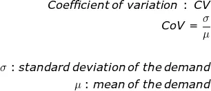
A demand distribution can be considered volatile when CV > 1.
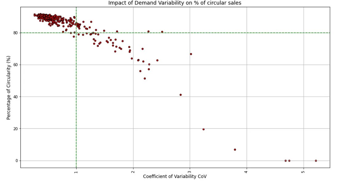
What is the variability of the 400 items included in the scope?

💡 Insights
- 99.9% of items with CV<1 have a percentage of circularity sales higher than 80%
- However, some items with CV > 1.5 have a percentage of circularity higher than 70%.
Logically, we can see the impact on the emissions reduction per item rented,
💡 Insights
- 100% of items with CV<1 have a reduction higher than 30 kg CO2e per Unit Rented.
As we do not control the demand variability, let's explore increasing the emissions reductions by changing the rental period.
Simulation with several rental periods
In the previous section, we simulated a rental period of 7 days.
We can now run the model with rental periods between two and twenty-eight days.
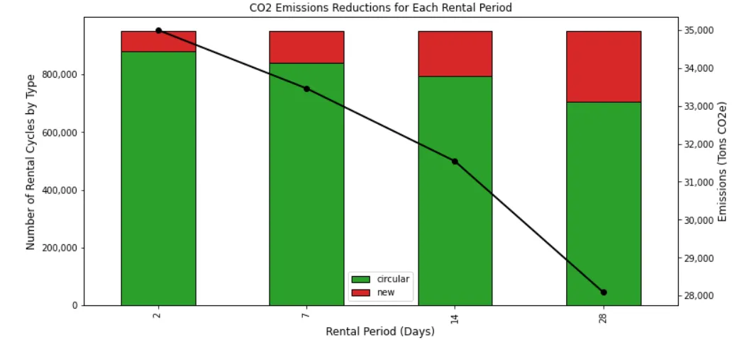
💡 Insights
- The reduction level drops when you increase the rental period.
- The optimal rental period is 2 days, with emissions cut reaching 35k Tons CO2e.
- Increasing the rental period reduces the percentage of circular items used.
This can be verified by looking at the percentage of circularity of items with a rental period of 2 days,
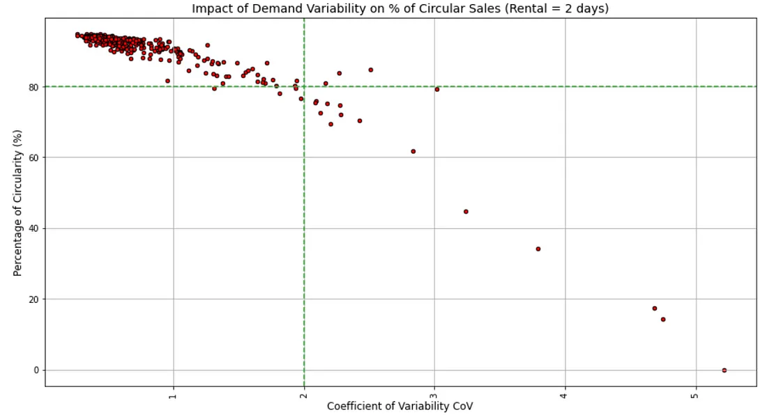
💡 Insights
- 99% of items with CV < 2 have more than 80% of their rental transactions fulfilled with reused items (versus CV<1 for rental period = 7 days)
That means a short rental period provides more flexibility in dealing with demand variability.
Without any surprise, we can see the same trend with the amount of water saved,
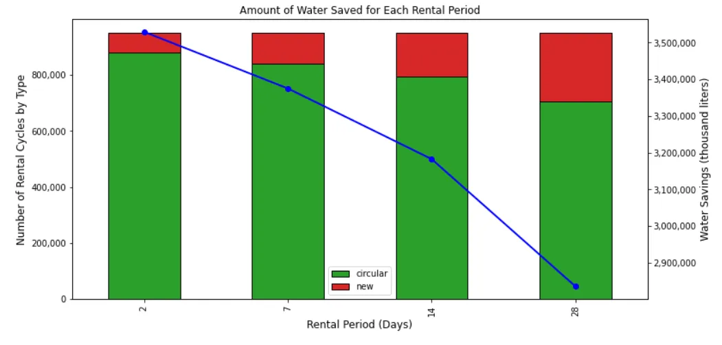
With longer rental periods, item availability for a rental is dropping.
Thus, you are losing inventory flexibility to absorb demand variability.

However, your circular model's performance remains impressive for a rental period of 28 days (60% CO2 reduction vs. a linear model).
This table can help to drive discussions and find the balance between commercial requirements and sustainability targets.
Circular Economy App
A light version of this model has been deployed on a web app: LogiGreen App
This prototype, currently in development, is already available for test.
How to test it?
You can test the model without uploading data by just following the steps below
Step 1: Go to the sustainability page
- 🔗Link: Sustainability Module
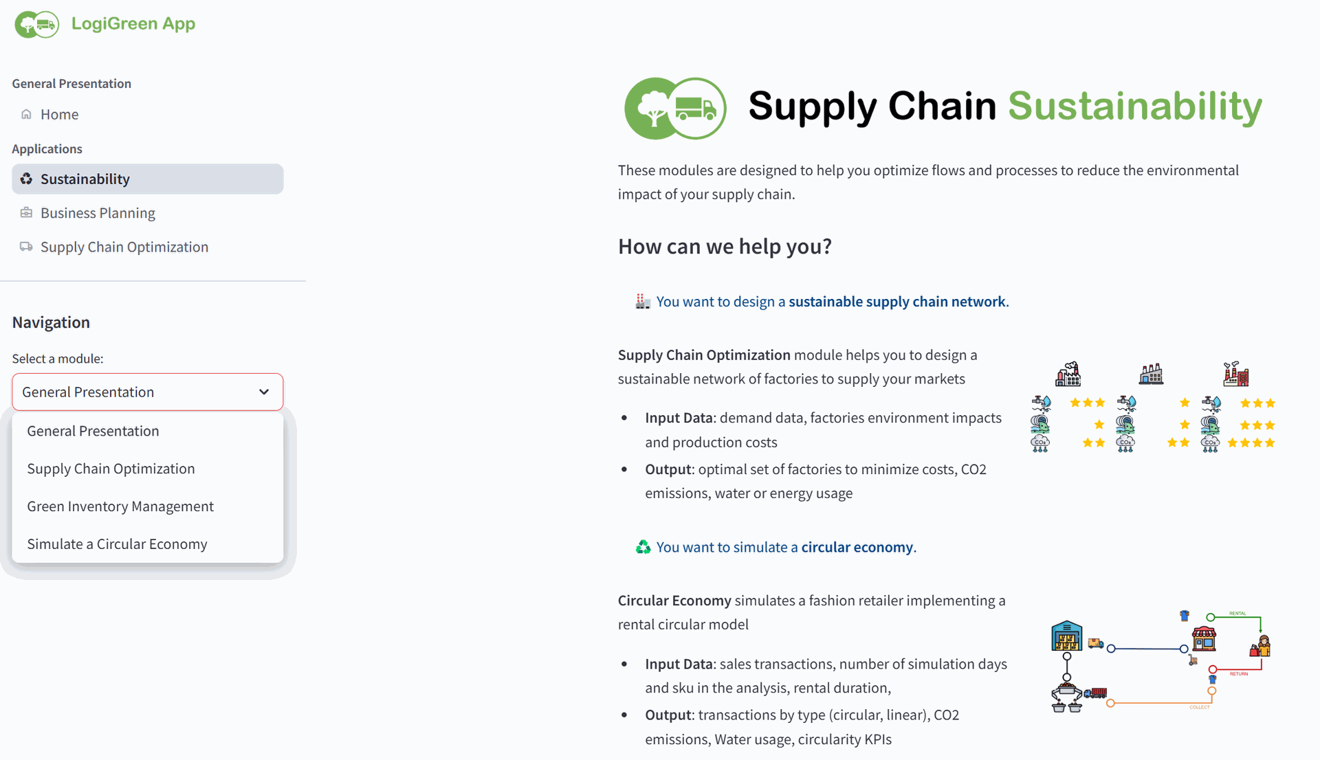
Step 2: Select 'Simulate a Circular Economy' on the side bar
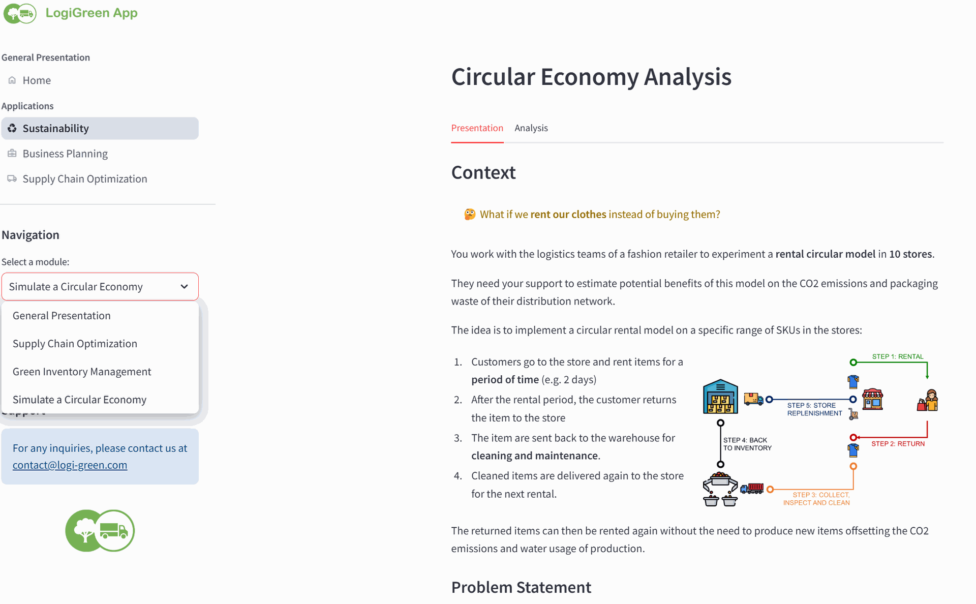
Step 3: Go the 'Analysis' tab
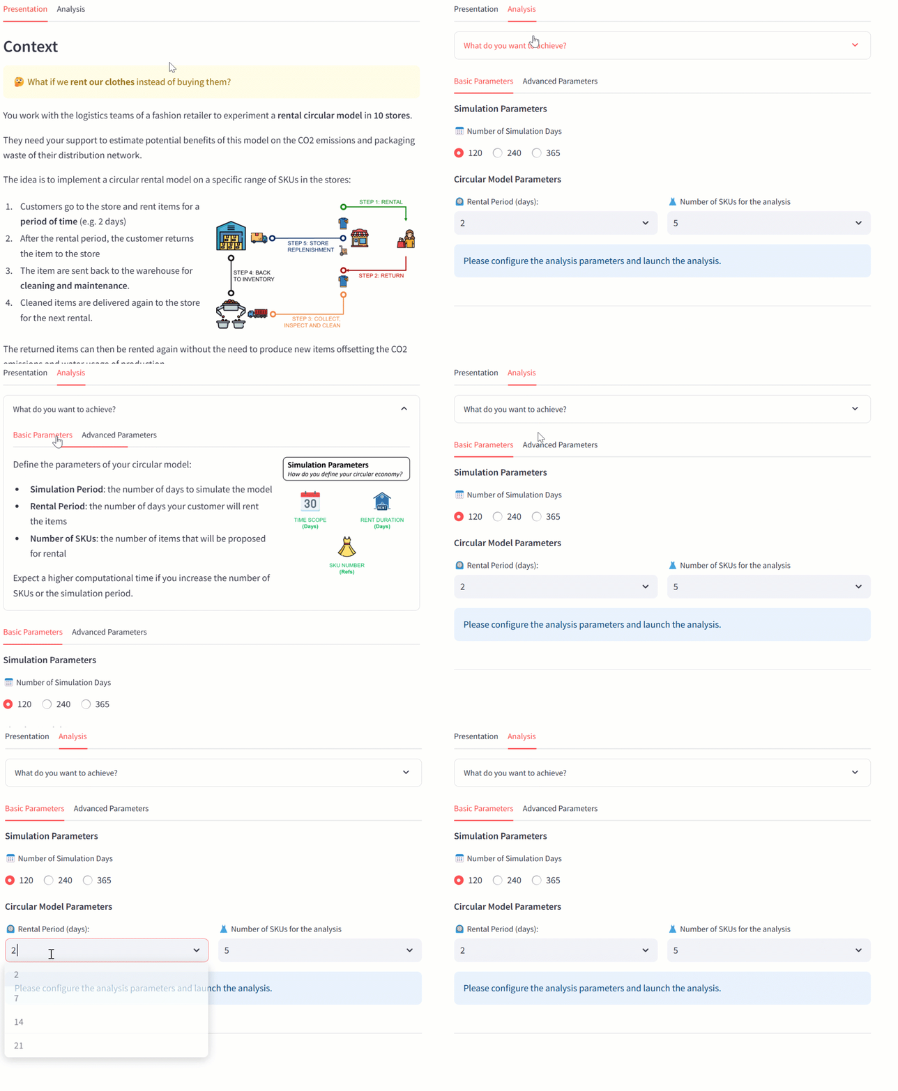
You can select
- Number of Simulation Days
- Number of SKUs
- Rental Period: days your customers rent your products
- Return Lead Time: days to send a return item back to the warehouse
- Cleaning Lead Time: days it takes to clean and refurbish returned items
- Delivery Lead Time: days to send cleaned items back to the store
Step 4: 'Launch the Analysis'
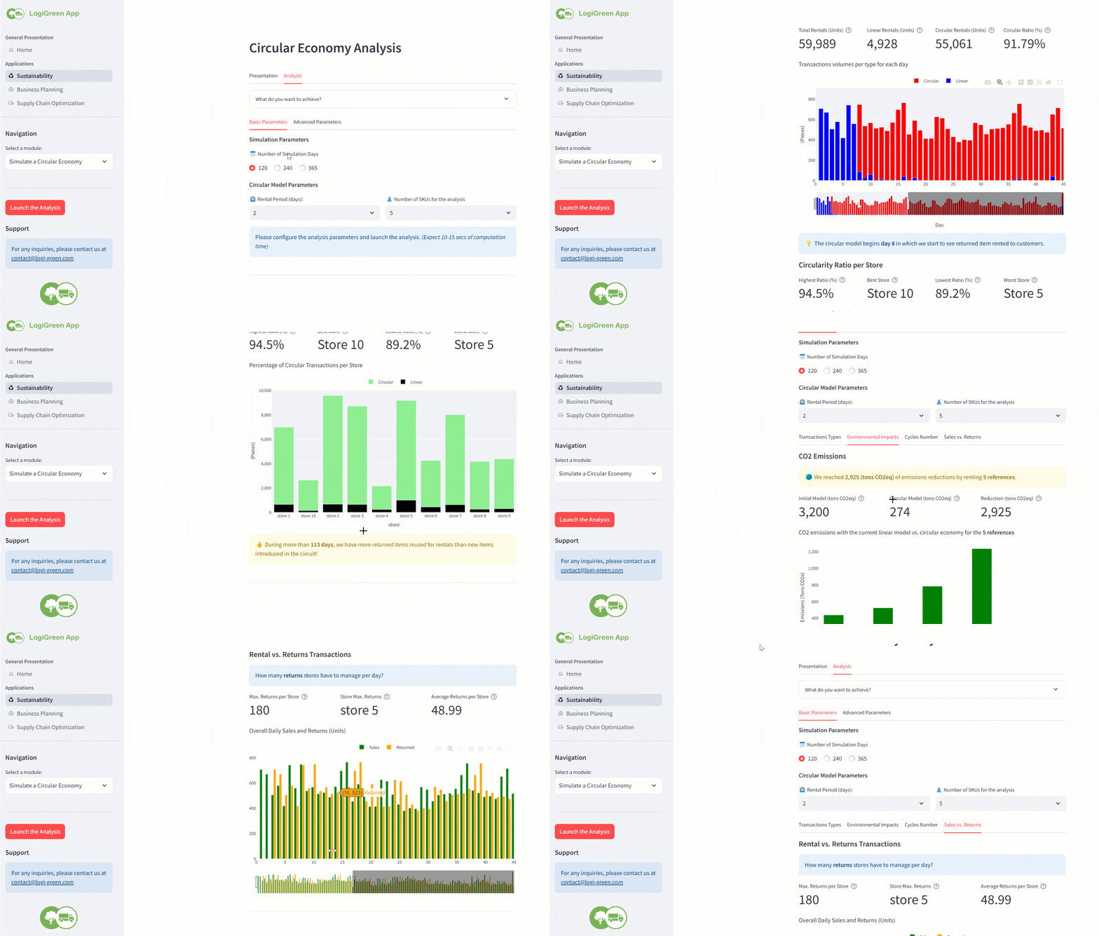
You will find multiple visuals for operational, costs and sustainability indicators.
Do not hesitate to refresh if you face a problem.
Any question?
For any inquiries, please contact us at contact@logi-green.com
This blog post is based on articles originally published on Medium