The master production schedule is the primary communication tool between the commercial team and production.
Production planning is a critical process for any manufacturing operation, but balancing the competing priorities of minimizing inventory costs and maximizing production efficiency can be challenging.
Can we automatically support your planning team to plan production batches?
This is a powerful tool for supply chain professionals because it can find the optimal balance between inventory and production costs.
In this article, we will discover how to use the Wagner-Whitin algorithm with Python to minimize the total cost of production.
Production Planning with Python
Scenario
We support a production planning manager in a small factory that produces radio equipment for local and international markets.
Customers send purchase orders (PO) with quantities and expected delivery dates to your commercial team.
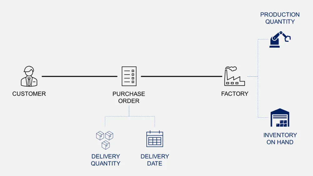
Your role is to schedule production to deliver on time with a minimum total cost of production that includes
- Setup Costs: fixed costs you have each time you set up a production line
- Production Costs: variable costs per unit produced
- Holding Costs: cost of storage per unit per time
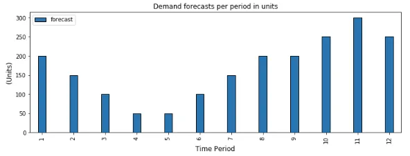
In our example, the customer ordered products for the next 12 months
What do we have to consider in the balance?
Setup vs. Inventory Costs
The main challenges for you are
- Reducing the average inventory on hand to minimize storage costs
- Minimize the number of production setups
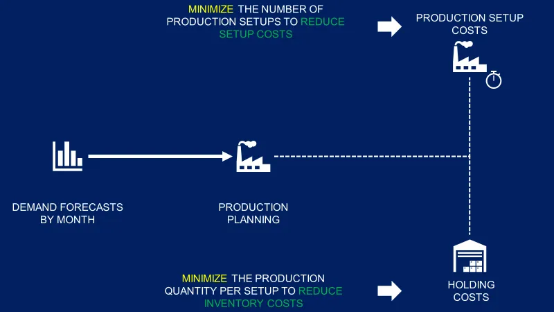
However, these two constraints are antagonistic.
Therefore, you need help finding an intuitive way to build an optimal plan.
Example 1: Minimize Inventory
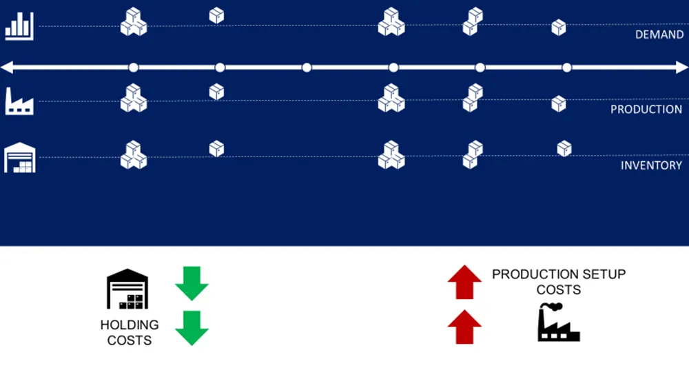
In this example, you produce the exact demand quantity each month
- Pros: No excess inventory
- Cons: You get production set up for each month with a positive demand
Example 2: Minimize the number of production setups
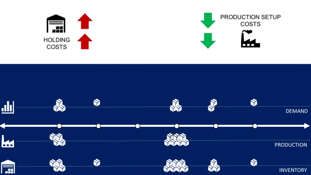
In this example, you build stock to minimize the number of setups
- Pros: only two production setups for the whole period
- Cons: a large stock on hand that increases the inventory costs
Conclusion
It would be best to have an optimization algorithm to balance the two constraints.
Solution
Assumptions
Suppose you receive a purchase order for the next 12 months with the quantities presented in the chart above.
- Set up cost: 500 $
- Holding cost: 1 $/unit/month
- Production cost per unit: 50 $/unit
- Units produced month m can be shipped the same month
- Inventory costs are charged from the month m+1
Have you heard about the economic order quantity?
Wagner-Whitin Algorithm
This problem can be seen as a generalization of the economic order quantity model that considers that demand for the product varies over time.
Wagner and Whitin developed an algorithm for finding the optimal solution by dynamic programming.
What’s the principle?
The idea is to understand each month whether adding the current month's demand quantity to past months' orders is more economical than setting up a new production cycle.
It starts with forward calculation …
Forward Calculation
Start at period 1:
- Calculate the total cost to satisfy the demand of month 1, D(1)
Period N:
- Calculate the total cost to satisfy the demand of month t, D(t)
- Look at all past orders (t=1 .. N) and find the cost for ordering for D(t) by adding the quantity to past orders D(t-1)
- Take the most economical option and go to t = N+1
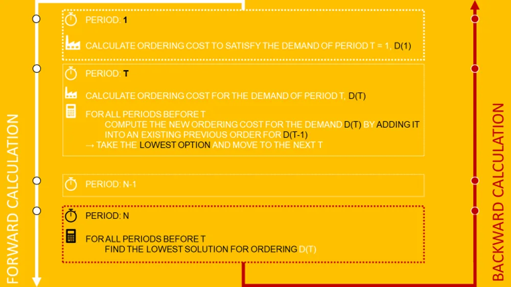
And to finish …
Backward Calculation
Start from period t = N and work backwards to find the lowest options to satisfy the demand of each D(t).
Let’s see how it looks like with an actual example.
Results & Conclusion
Forward Calculation
You should export the results of the forward calculation using a table like the one below:

Let me take a few examples:
Period 1, if you produce for the
- First month demand only (D(1) = 200 units): 500$
- Two first months (D(1) + D(2) = 350 units): 650$
Now, let’s finish with the backward calculation.
Backward Calculation
We can use the table above to resolve the algorithm visually using the rules explained before.

- Start with t = 12
The cheapest solution is to produce the month 11 for D(11) + D(12) - Continue with t = 10
The cheapest solution is to produce the month 9 for D(9) + D(10) - Continue with t = 8
The cheapest solution is to produce the month 6 for D(6) + D(7) + D(8) - Continue with t = 6
The cheapest solution is to produce the month 1 for D(1) + D(2) + D(3) + D(4) + D(5) + D(6)
What’s the result?
Final Solution
- Month 1: Produce 550 units to meet the demand of the first five months
- Month 6: Produce 450 units for months 6, 7 and 8
- Month 9: Produce 450 units for months 9 and 10
- Month 11: Produce 550 for months 11 and 12
Inventory Optimization
The chart below shows the inventory on hand (IOH) can be way higher than the demand forecast.
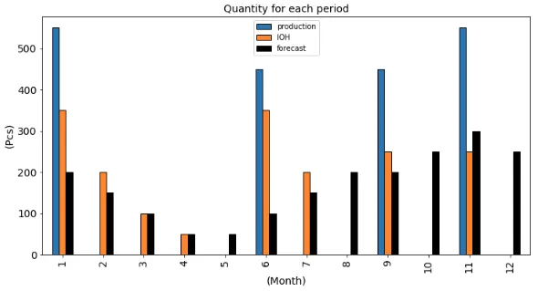
This shows no balance between setup and inventory impacts on the overall costs.
That means keeping a high inventory is way cheaper than multiplying the number of setups.
If the holding costs were higher, you would likely see an IOH closer to the forecasts and more production months.
A great balance between inventory and set-up costs.
In the chart below, you can follow the cumulative holding and set-up costs over the 12 months:
Holding Costs vs. Set-Up Costs after Using Wagner Within Algorithm for Production Planning
The algorithm balances inventory optimization and reduces the number of setups, as the cumulative value of holding and set-up costs is nearly equal.
What does that mean?
That means,
- If holding costs per unit are very high, the algorithm will increase the number of setups to minimize inventory.
- If you have very high costs per setup, the algorithm will tend more to build inventory in a minimum number of setup costs.
Do you want to try yourself?
Production Planning App
A prototype of this model has been deployed on a web app: LogiGreen App
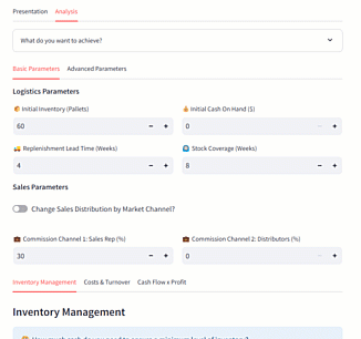
This prototype, currently in development, is already available for test.
How to test it?
You can test the model without uploading data by just following the steps below
Step 1: Go to the supply chain optimization page
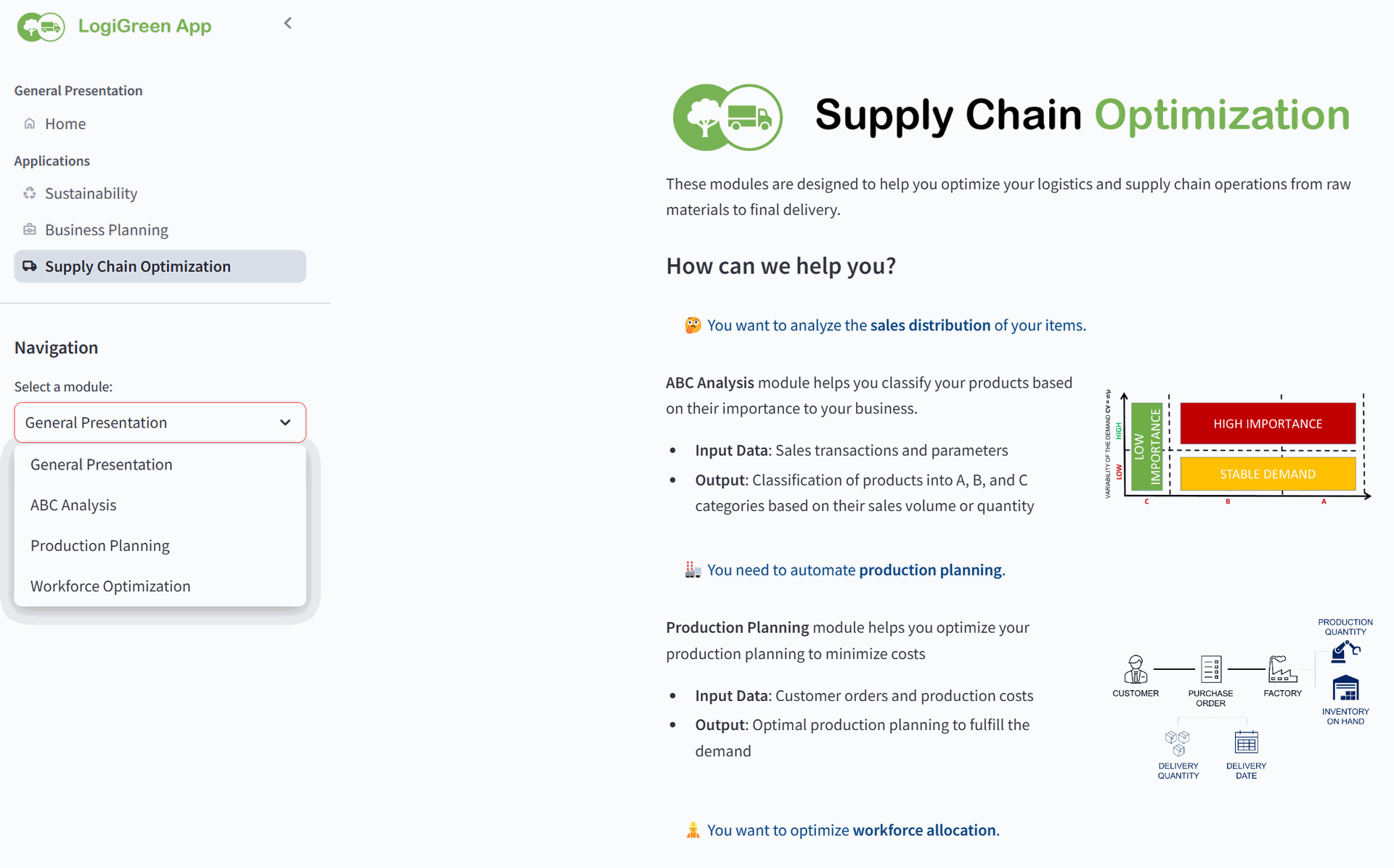
Step 2: Select 'Production Planning' on the left side bar
You will arrive in the presentation page of the module where you can find a brief presentation of the model with the inputs parameters and the results provided.
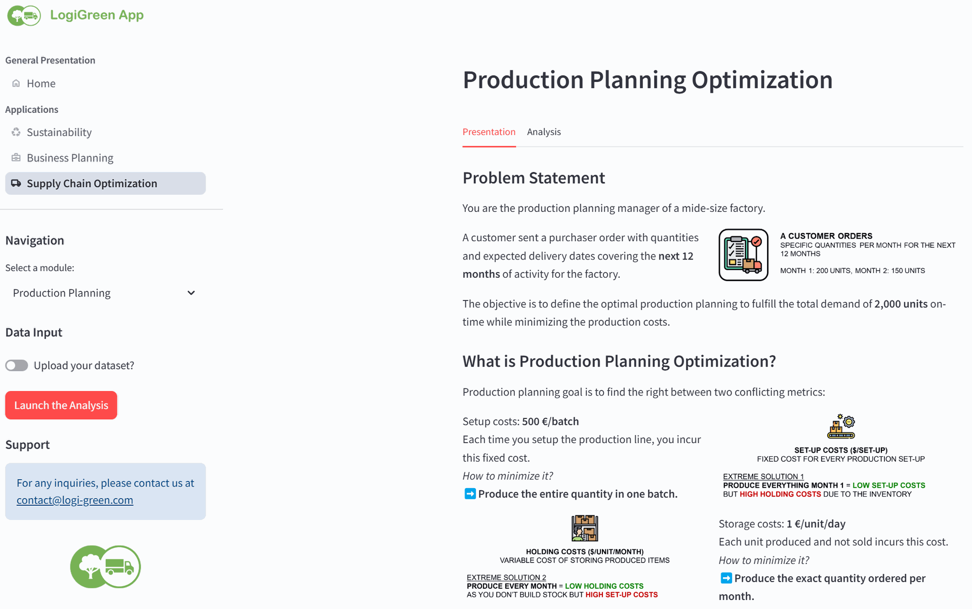
Step 3: Go to the 'Analysis' tab
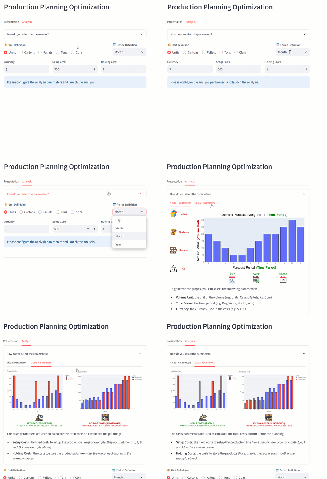
You can select
- Unit definition (Units, Cartons, Pallets, Tons or Cbm)
- Time period (Day, Week, Month or Year)
- Setup Costs ($/Setup)
- Hodling Cost ($/Unit/Period)
- Add constraints of maximum footprint
Step 4: Click on Launch the Analysis
You can then visualize the results.
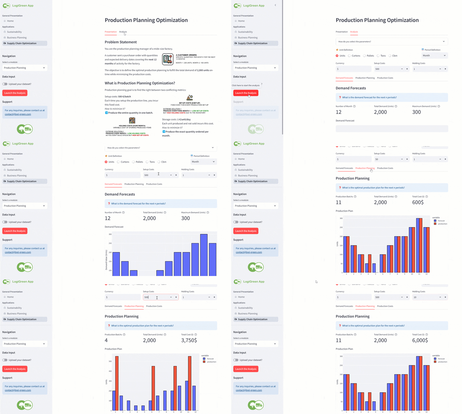
You will find additional indicators like the Cost of Goods Sold (COGS) along with other business metrics to help you assess the results.
Do not hesitate to refresh if you face a problem.
Any question?
For any inquiries, please contact us at contact@logi-green.com
This blog post is based on articles originally published on Medium
- Production Planning with Python by Samir Saci